During model selection, Pareto Smoothed Importance Sampling Leave One Out Cross-Validation (PSIS-LOO-CV), approximated out of sample predictive density where LOO-CV were not reliable (flagged observations, in this case, reports). Out of ten species (eleven species including models for wild boar including wildlife accidents), seven species had less than ten flagged observations (reports) with a Pareto k-value higher than 0.7. Rock ptarmigan, American mink and greylag goose had more than ten flagged observations with a Pareto k-value higher than 0.7 and were further excluded from exact leave one out cross-validation.

Evaluation of predictive performance was performed by examining the difference in expected log-pointwise predictive density (ELPD) and standard error (SE) (ELPD/SE). The higher difference between ELPD and SE, the better predictive ability for other datasets. For nine of out ten species, the full covariate model ranked highest of the four models (Table 2). The reduced covariate model ranked highest for greylag goose.

The full covariate model only had a pronounced effect for beaver and wild boar (excluding wildlife accidents) with a SE four times smaller than ELPD (Table 2). For wild boar (including wildlife accidents), red fox, mountain hare, and common eider, with a SE two to three times smaller than ELPD, there was weak support that the covariate model would perform better with other datasets. Finally, for nine of out ten species, at least one covariate had an effect on harvest estimates. For rock ptarmigan, covariates did not have an apparent effect on harvest estimates (Table 2).

All game species were initially tested with all 15 covariates (16 for wild boar, including wildlife accidents). However, if any credible interval overlapped with zero or there was a correlation between covariates, these covariates were removed.

For nine out of ten species, at least one covariate had either a positive or negative effect on harvest estimate (Figure 1, Table 2). For example, a positive effect of temperature on harvest estimate indicates that the higher temperature within an HMP, the more harvest there is for respective species. A positive effect of West/East (gradients) indicates that the further east in Sweden, the more harvest there is for separate species. Suppose the credible interval is close to zero. In that case, there is an effect of that covariate on harvest estimate, however vague. If the credible interval is further away from zero, there is a strong effect on the covariate on harvest estimate.

For most of the game species, the effect of covariates was quite expected. However, there were both expected and unexpected results for mountain hare and wild boar or, more likely contradictory results. In the figure for mountain hare, one can see two clear north and south gradients, precipitation, and humidity. These two covariates imply that the more precipitation and humid it is, the more mountain hare is felled, which was expected since mountain hare is mainly located in northern Sweden. However, the result also shows that more mountain hare is felled in southern Sweden. As for wild boar (including and excluding wildlife accidents), the covariates water and coastline sea/lake/river both had a positive and negative effect. One possible explanation for these errors is that there could be a correlation between covariates (covariates are very alike), which can contribute to a complicated variation of several factors. 

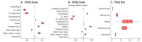
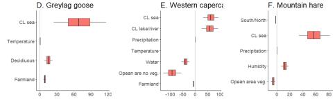
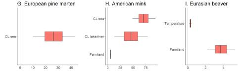
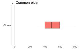
Figure 1: Boxplot over covariate effect on hunting of A. wild boar, B. wild boar including wildlife accidents, C. red fox, D. greylag goose, E. western capercaillie, F. mountain hare, G. European pine marten, H. American mink, I. Eurasian beaver, and J. common eider. The plot shows the 95 % credible intervals, where the box represents 50 % of all values and the distance between the percentiles. The black line inside the box indicates the median, and the dashed line outside the box represents outliers. A negative/positive effect indicates less/more hunting for the respective covariate. Abbreviations: veg = vegetation, temp. = temporary, CL = Coastline. 

During posterior prediction on unreported areas, all parameters from earlier steps were used to predict how much has been hunted in the unreported areas. 

The coefficient of variation (CV), calculated from each HMPs predictive posterior mean and standard deviation for both the covariate and null model, was compared for each HMP and county (Figure 5). The comparison was made by evaluating the ratio between CV between the two models (CV of null model/CV of covariate model), where a positive value indicates that the CV was higher for the null model, and a negative value indicates that the CV was higher for the covariate model.

For all species, the covariate model had a smaller value of CV than the null model, wild boar (169/243), wild boar (including wildlife accidents) (186/243), red fox (265/306), greylag goose (278/298), Western capercaillie (202/271), American mink (298/306), Eurasian beaver (151/249), common eider (55/76), mountain hare (154/306), and European pine marten (179/301).